Python Tools for Kurtosis Calculation
Read Time:3 Minute, 56 Second
In this comprehensive tutorial, let’s delve into the topic of kurtosis computation in Python, providing an in-depth exploration of the statistical measure’s calculation, interpretation, and practical applications within data analysis.
It primarily serves as a metric for characterizing the shape of a probability distribution, specifically addressing its “tailedness.” This statistical measure assesses the relative thickness or thinness of a distribution’s tails when compared to a standard normal distribution.
While skewness focuses on distinguishing the tails of a distribution by examining extreme values or assessing tail symmetry, kurtosis takes a different approach. It determines whether there are significant extreme values in either tail of the distribution or simply gauges whether the tails exhibit heaviness or lightness.
To continue with this tutorial, you’ll need to have the ‘scipy’ Python library at your disposal. If it’s not already installed, please open the “Command Prompt” (on Windows) and execute the following code for installation:
pip install scipyExploring Kurtosis in Statistics
In the realm of statistics, kurtosis serves as a crucial metric for understanding the shape and characteristics of a probability distribution. Essentially, it tells us how “peaked” or “flat” the distribution is, and it provides insights into the thickness or lightness of its tails. It value offers valuable information about the degree to which the tails of a particular probability distribution deviate from those of a standard normal distribution.
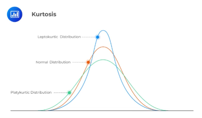
Kurtosis can manifest in various numerical values:
| Kurtosis Type | Description |
|---|---|
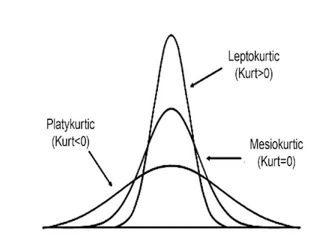
| Positive Excess Kurtosis | When (kurtosis – 3) is positive, it signifies a sharply peaked shape, and the distribution is leptokurtic. |
| Negative Excess Kurtosis | When (kurtosis – 3) is negative, it suggests a flatter peak, and the distribution is classified as platykurtic. |
| Zero Excess Kurtosis | When (kurtosis – 3) equals zero, it closely resembles a normal distribution and is termed mesokurtic. |
Below is a tabular summary of the information presented above:
| Type | Kurtosis | Excess Kurtosis |
|---|---|---|
| Leptokurtic | >3 | >0 |
| Platykurtic | <3 | <0 |
| Mesokurtic | =3 | =0 |
A Step-by-Step Guide to Calculating Kurtosis
Calculating kurtosis might seem complex at first, as it involves finding the fourth standardized moment of a distribution. However, fear not! Follow the steps below to gain a comprehensive grasp of the calculation process.
The kth moment of a distribution can be computed using the following formula:
- μ˜k=μkσk=E[(X−μ)k](E[(X−μ)2])k2
As previously discussed, skewness corresponds to the fourth moment of the distribution and can be determined using the following formula:
- K=m4(m2)42=m4(m2)2
Considering that the second moment of the distribution represents its variance, the preceding equation can be streamlined to:
- K=m4(σ2)2
In this context, where:
- mk=1N∑n=1N(xn–x¯)k
Example:
There are quite a few formulas discussed above. To make these concepts more comprehensible, let’s illustrate them with an example!
Imagine you have the following sequence of 10 numbers, which represent students’ grades on a test:
- X = [55, 78, 65, 98, 97, 60, 67, 65, 83, 65]
Calculating the mean of X yields: x̄ = 73.3.
Now, let’s compute m4:
- m4=110∑n=110(xn–x¯)4
- m4=(55−73.3)4–(78−73.3)4–…–(65−73.3)410=85,630.5
Solving for m2:
- m2=110∑n=110(xn–x¯)2
- m2=(55−73.3)2–(78−73.3)2–…–(65−73.3)210=204.61
Solving for K:
- K=m4(m2)42=85,630.5(204.61)2=2.045373
Calculating Kurtosis in Python
In this section, we’ll walk you through an illustrative example of calculating kurtosis using Python.
To begin, let’s construct a list of numbers similar to what we used in the previous section:
- x = [55, 78, 65, 98, 97, 60, 67, 65, 83, 65]
To compute the Fisher-Pearson correlation of skewness, you’ll require the scipy.stats.kurtosis function:
- from scipy.stats import kurtosis;
- print(kurtosis(x, fisher=False)).
And the expected result should be:
- 2.0453729382893178
Note: By setting fisher=False in the provided code, you calculate the Pearson’s definition of kurtosis, where the kurtosis value for a normal distribution equals 3.
For the given sequence of numbers, the calculated kurtosis is approximately 2.05, and the excess kurtosis is approximately -0.95. These values indicate that the distribution has thicker tails and is flatter than the normal distribution.
Conclusion
In this article, we’ve explored the process of calculating kurtosis for a dataset in Python, leveraging the capabilities of the SciPy library. By delving into the intricacies of kurtosis and its various definitions, we’ve equipped you with the knowledge and tools to assess the shape and tails of probability distributions. Armed with this understanding, you can better analyze and interpret data in a wide range of statistical applications.
Happy
0 %
Sad
0 %
Excited
0 %
Sleepy
0 %
Angry
0 %
Surprise
0 %


Average Rating